Model Reduction:
The Manifold Boundary Approximation Method

Removing Parameters from Sloppy Models

Sloppy models have lots of parameters and most of them cannot be inferred from data. Statistical uncertainties in the inferred values are often huge, even infinite. You might wonder, why don't we just remove the sloppy parameters from the model? In other words, why don't we simplify or reduce the model to include only the important pieces?

Simple models are a powerful tools for understanding the behavior of a physical system. In fact, science is full of examples of mathematical models that are simple descriptions of otherwise complex processes. Because these models concisely illustrate the important parts of the system, they vividly illustrate the physical mechanisms that control the system. In fact, identifying which are the control mechanisms is a large part of complex systems research.

Unfortunately, simplifying models in a way that reveals the important parts and ignores the unimportant pieces is a very difficult problem. There are several challenges to doing this generally for sloppy models.

1. It is often combinations rather individual parameters that are important
2. These combinations are often nonlinear functions of parameters
3. Even if the right nonlinear combination could be found, how do you remove it from the model?

To overcome these challenges, we developed a new approach to model reduction based on our geometric understanding of models. We call this method the Manifold Boundary Approximation Method (MBAM).

Manifold Boundaries

By thinking about models geometrically, we can better understand how a model reduction scheme ought to work. Although sloppy models have many parameters, their behavior exhibits a low-effective dimensionality. This low-dimensionality is quantified by the hyper-ribbon structure of the model manifold. Just as a ribbon is a three-dimensional object that can be approximated by a two-dimensional surface or even a one-dimensional curve, we would like to approximate our hyper-ribbon by an object of lower dimension.

The approach we ultimately decided to use was to use the boundary of the model manifold itself as an approximation. Superficially, the boundaries make a nice approximation scheme since they naturally follow the curvature of the original model manifold. However, what makes the boundary approximation method so powerful are the physical interpretations that can be attached to the new, simplified models.

To illustrate, consider what happens to a geodesic curve as it approaches the boundary of a model manifold. Geodesics curves are approximately straight lines on the model manifold, but correspond to highly nonlinear curves in parameter space. As these curves approach a manifold boundary, however, several things happen that make indicate the boundaries of the manifold have special physical meaning.

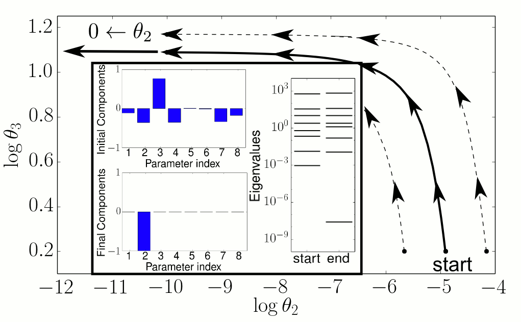
First, as they approach a boundary the geodesic paths in parameter space stop bending and straighten out as in the figure below. Second, although the initial direction of the geodesic may have involved a complicated combination of parameters, as it approaches a boundary it rotates into a simple, physically relevant combination. Finally, as the geodesic approaches the boundary, the smallest eigenvalue of the Fisher Information, peels away from the others and approaches zero.

These three observations about the geodesics as they approach a boundary indicate that the boundaries correspond to limiting approximations of the model. In the figure above, for example, the boundary corresponds to the limit that the second parameter becomes zero. The physical meaning of the boundaries vary with the model. They might correspond to chemical reactions equilibrating or saturating in systems biology. They may correspond to removing high-frequency fluctuations in the Ising model. Whatever the model, the boundaries always correspond to limits that can be given simple, physical interpretations.

The Manifold Boundary Approximation Method

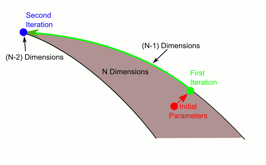
Understanding the nature of the manifold boundaries enables an approach to model reduction that we call the Manifold Boundary Approximation Method (MBAM). By approximating the original model manifold with the boundary along the most narrow width, we retain most of the predictive power of the original model while removing the least important parameter combination. The new approximate model is only marginally less sloppy than previous, but it can likewise be simplified in the same way. MBAM therefore consists of this four step iterative algorithm:

1. Find the (locally) least important parameter combination from the eigenvalues of the FIM.
2. Follow a geodesic path oriented along this direction until the manifold boundary is discovered.
3. Identify the limiting approximation corresponding to this boundary and explicitly evaluate it in the model.
4. Calibrate the new model by fitting its behavior to the behavior of the original model

The MBAM Algorithm.

Iterating these four steps removes parameter combinations one at a time until the model is sufficiently simple. What constitutes "sufficiently simple" will vary based on context. The final model will then correspond to a hyper-corner of the original model manifold.

The manifold boundary approximation method naturally overcomes the three challenges to model reduction listed above. By repeatedly evaluating limiting approximations in the model, the irrelevant parameters are removed and the remaining parameters naturally group into the physically important combinations. These combinations are often nonlinear combinations of the original bare parameters. MBAM naturally connects microscopic physics with emergent, macroscopic physics in a semi-automatic way. This is perhaps best illustrated by an example.

Systems Biology Example

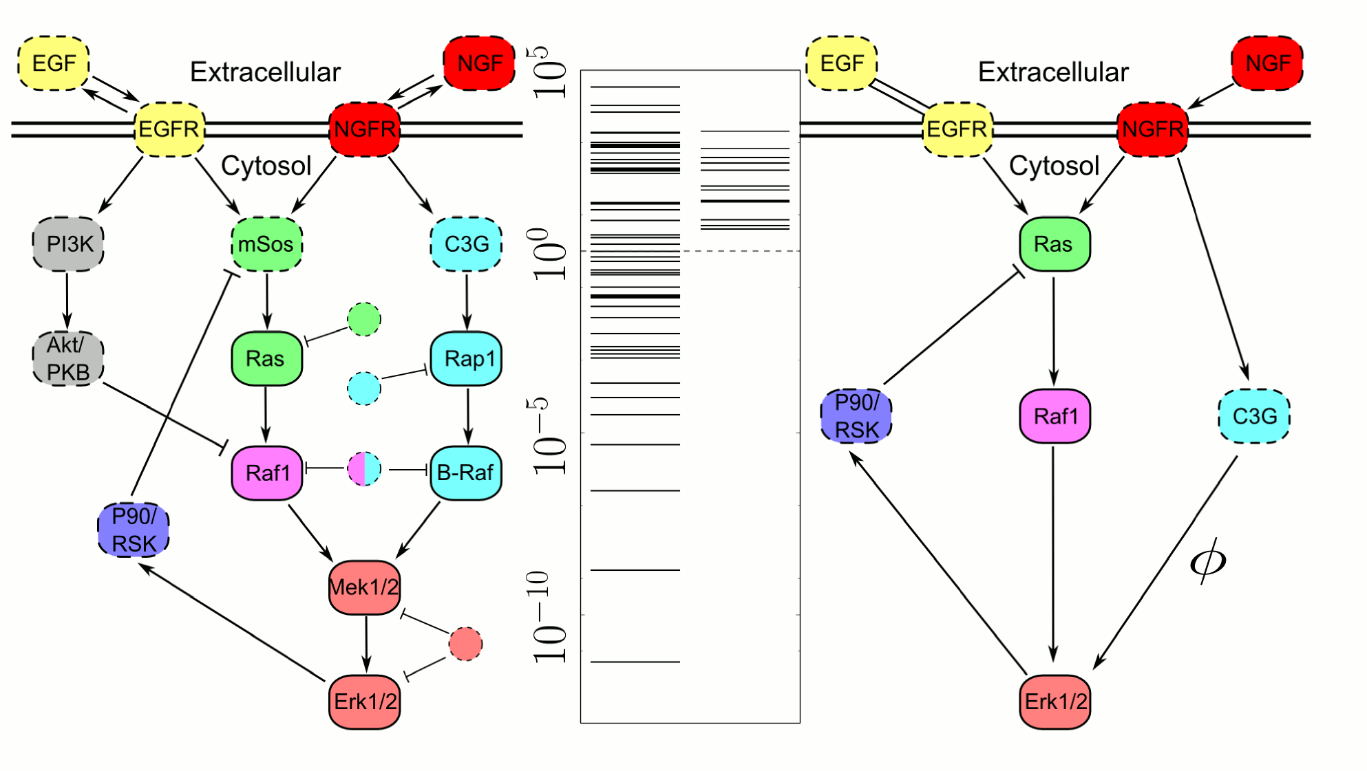
One of the first models to be identified as sloppy was a systems biology model describing signaling in a developing rat cell. This particular model had 48 parameters and 29 differential equations. However, because the model was made of many inhomogeneous components interacting in highly nonlinear ways, it was not obvious which parameter combinations were important nor could any of the traditional model reduction methods be used to simplify it. MBAM, however, was able to identify a series of limiting approximations that could be applied to the model. The result was a new effective model that had only 12 parameters and 6 differential equations.

Original and Simplified PC12 Network Diagrams.

The figure shows the network diagram for the original model and the new, effective diagram for the simplified model. Notice how most of the superfluous components have been removed. What remains is a dramatic illustration of the negative feedback loop (from Erk to P90/RSK to Ras) that is the mechanism responsible for the system behavior. Qualitatively, this negative feedback loop is how the biologists had understood the behavior of the system. MBAM naturally recovered the same result and produced a quantitative, mathematical model to describe this interpretation in the process. What remains after the simplifying process are precisely the 12 parameters that are necessary for the model to be predictive. This can be seen by noting that there are no small eigenvalues in the FIM for the new model. All the sloppy parameters (combinations) have been removed and all of the stiff parameter (combinations) have been kept!

The nice thing about the approximate model is that it is not just a "black box". Instead, it explains the system's collective behavior in terms of the components of the original model. For example, consider the effective interaction between C3G and Erk in the new model. The strength of this interaction is controlled by a parameter (labeled \(\phi\) in the diagram). This parameter has a definition in terms of the original model parameters that emerges through the sequence of limiting approximations: $$ \phi = \frac{ (\mathrm{k_{Rap1ToBRaf}}) (\mathrm{K_{mdBRaf}}) (\mathrm{k_{pBRaf}}) (\mathrm{K_{mdMek}}) }{ (\mathrm{k_{dBRaf}}) (\mathrm{K_{mRap1ToBRaf}}) (\mathrm{k_{dMek}}) }.$$ This parameter is the "renormalized" parameter of the effective model. Notice that it is a nonlinear combination of 7 other parameters. Each of the seven parameters can influence the behavior of the model but only through their effect on \(\phi\).

Since this model has 12 parameters, there are 11 other expressions (of varying complexity) similar to the one for \(\phi\) above. Each one of these parameters controls an important feature in the model's behavior. In fact, if the simplified model were fit to data, all of the parameters could be inferred with small error bars (notice the eigenvalues of the simplified model in the figure). The new model is not sloppy!

Unifying Model Reduction Methods

The manifold boundary approximation method makes very few assumptions about the model. We have seen that it performs spectacularly on our systems biology model. To what other models can it be applied in what contexts?

At its heart, MBAM is a tool for identifying limiting approximations. There are a wide variety of model reduction techniques that have grown up searching for these types of approximations in different contexts. For example, in dynamical systems, singular perturbation theory explores the behavior of differential equations in the limit that one of the time scales is much faster than the others. If there is a parameter in the model that explicitly controls the time scale, then the limit that that parameter becomes zero will correspond to a boundary of the model manifold. Therefore, singular perturbation theory can be recovered as a special case of the MBAM procedure.

Many other approximation techniques can similarly be subsumed as special cases of the MBAM procedure. Continuum limits and thermodynamic limits are two other obvious examples of a limiting approximation. However, other approximation methods that are not obviously limiting approximations can similarly be reproduced by MBAM. For example, the renormalization group, a powerful tool in statistical physics, as well as balanced truncation, the cornerstone of dynamical systems order reduction in control theory, both can be recovered as special cases of MBAM.

MBAM provides a new way to think about model reduction that is very general. By unifying and generalizing many time-tested model reduction techniques, it is a step toward a unified theory of model reduction.

h