Sloppy Curvature

Intrinsic Properties of Sloppy Models

Our initial explorations of sloppy models using differential geometry revealed that sloppy models had a common global structure that we called a hyper-ribbon. It was a bounded hyper-surface with a hierarchy of widths. The hierarchy of widths was exactly analogous to the hierarchy of eigenvalues that had been observed in many multi-parameter models. However, unlike the eigenvalues that can be manipulated by reparameterizing the model, the hierarchy of widths is an intrinsic feature of the model. We now ask the question: are there any other features of sloppy models that are true for all parameterizations? In particular, we were curious about the curvature, since it is a quantity that is important mathematically.

Measures of Curvatures

There are many different measures of curvature. Here we summarize them briefly before discussing their relation to sloppy models. Although these three quantities are all related to the nonlinearity of the model, they represent very different concepts. We don't give any formulas here, but will try to describe qualitatively what these curvatures mean.

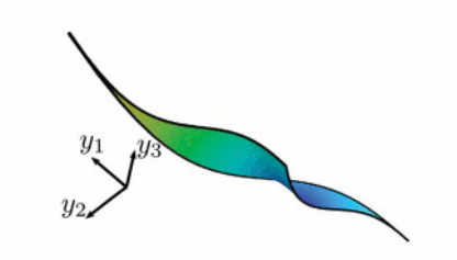An example of intrinsic and extrinsic curvature.

Intrinsic Curvature is a measure of curvature with which physicists are often familiar since it plays a central role in general relativity. It is a measure of nonlinearity that is intrinsic to the manifold in the sense that it is the same regardless of how the manifold is parameterized or how it is embedded in higher-dimensional spaces -- in fact, calculating intrinsic curvature makes no reference to embedding spaces. This curvature turns out to be not so useful for modeling since the embedding space (i.e. the data space) plays such an important role. Instead, we will be primarily interested in the extrinsic curvature.

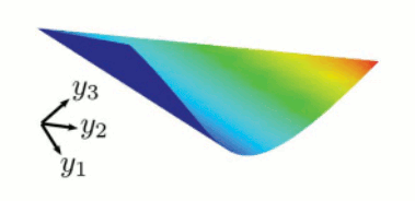An example of a surface with extrinsic but no intrinsic curvature.

Extrinsic Curvature is a measure of curvature that describes how the manifold is embedded in a higher-dimensional space. If a manifold has a non-zero intrinsic curvature, it will also have an extrinsic curvature, but the inverse is not necessarily true. A model with extrinsic curvature but no intrinsic curvature is an example of a ruled surface. An example is a two parameter model with one linear and one nonlinear parameter (such as an amplitude and an exponential rate in the figure to the right). For many models, it turns out that the extrinsic curvature is very small, especially when compared to the widths or the parameter-effects curvature.

Parameter-effects Curvature is not really a measure of curvature in the usual sense. It is a term invented by statisticians studying the nonlinearity of models to encompass all of the nonlinearity that could in principle be removed by a reparameterization. Although this "curvature" is not intrinsic to the model since it can be removed by the right choice of parameters, it turns out that nearly all models have much larger parameter-effects curvature than extrinsic curvature. Below, we explain why this is by using our paradigm that models are just interpolation schemes and later use this fact to improve numerical methods for finding best fits.

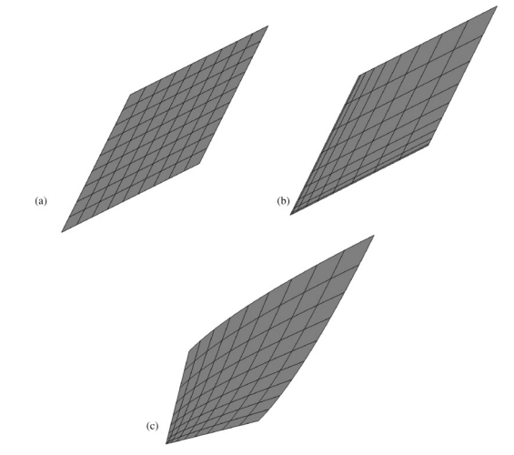Three parameterizations of the plane. a) A skewed coordinate system with no parameter-effects curvature. b) A coordinates-system exhibiting a compression parameter-effects curvature. c) Rotating coordinates are another type of parameter-effects curvature. In higher dimensions, a third type of parameter-effects curvature exists known as torsion which describes twisting of coordinates.

Hierarchy of Curvatures

Of course, there are formulas for calculating each of the curvatures described above which you can find in our paper. Using these formulas we calculated the extrinsic and parameter-effects curvatures for different models corresponding to different directions on the manifold. It turns out that these measures of curvature correspond to an inverse distance, so we can actually compare the curvatures to the widths of the hyper-ribbons in each of the sloppy directions as we do in the picture below.

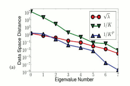Sloppy eigenvalues, extrinsic curvatures, and parameter-effects curvatures. The inverse extrinsic curvatures (1/K) and inverse parameter-effects curvatures (1/Kp) are both logarithmically spaced just like the hyper-ribbon widths, but with twice the slope. Also, the parameter-effects curvatures are much larger than the extrinsic curvatures in any direction.

In the picture above you can see that the curvatures are highly anisotropic. Curvatures are very large in the sloppy directions and much smaller along the stiff directions. This observations makes intuitive sense. Curvatures are roughly a measure of the bending of the manifold. More precisely, it is the amount of bending per distance moved on the manifold squared. Along sloppy directions, that distance moved can be very small (as measured by the sloppy eigenvalues), which has the effect of magnifying the curvature in these directions. In fact, the amount of the magnification seems to be exactly proportional to the eigenvalues of the metric tensor (least squares Hessian).

Interpolation and Curvatures

It turns out the observed hierarchy of extrinsic and parameter-effects curvature is also a general feature of sloppy models which we observe empirically. We can also use arguments from interpolation theory to explain this observation just as we did for the observation of the manifold widths.

To understand the curvature of sloppy models, first notice that if our model has N parameters, then we can reparameterize our model so that N independent data points are the parameters. We can also construct an interpolating polynomial (linear model) that matches the model predictions at these N data points. Using the same interpolation arguments as before, we then can say that the discrepancy between the true, nonlinear model and the linear approximation is bounded by an amount comparable to the smallest manifold width. We now assume this deviation from flatness varies smoothly along each width. We can check this assumption numerically, and it seems to hold fairly generally. From these assumptions, the extrinsic curvature should be given by K = ε/W², where ε is the deviation from flatness (roughly the smallest width) and W is the width in the given direction. Thus the curvatures should scale like the square of the widths, i.e. the inverse sloppy eigenvalues, exactly as observed. The largest curvature (along the narrowest width) should also be given by K = 1/W, i.e. should be given by the narrowest width since for this case ε=W. This is also exactly what is observed.

We now understand the extrinsic curvature. What about the parameter-effects curvature? If you look at the figure further up on the page illustrating parameter-effects curvature, you may notice that the parameter-effects curvature would be an extrinsic curvature on a lower-dimensional manifold, i.e. a manifold in which some of the parameters were held fixed. We can therefore understand parameter-effects curvature using many of the same arguments as extrinsic curvature. In particular, the observation that it scales as the inverse sloppy eigenvalues is obviously shared by both types of curvature. The difference between the two is only in the scale. We understand the scale of the parameter-effects curvature by noting that nearly all of the parameter-effects curvature is an extrinsic curvature when all of the other parameters are held fixed. We therefore expect the scale to be set by the widest width, i.e. the smallest width of a one-dimensional manifold, precisely what is observed. These ideas are summed in a simple caricature of a typical sloppy model manifold (below).

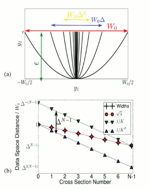Caricature of manifold cross sections. If we assume the bending of the manifold ε is uniformly spread out over the widths (above) then we can predict the scaling of the curvatures (below). Notice how well the caricature matches the actual widths/curvatures for a real model in the figure above.

Applications

From the arguments here and on the the previous page, we can put together a very clear idea of what the model manifold looks like. The dominant features are the boundaries which form a hierarchy of widths. The extrinsic curvature is very small compared to the size of the bare nonlinearities, which are given by the paramter-effects curvature. All of these facts are backed up both by numerical experiments on many models, as well as analytical arguments based on interpolation theory. Thinking of models as generalized interpolation schemes is very powerful!

Since most people doing nonlinear modeling are not familiar with differential geoemtry or the model manifold, it is probably not immediately clear what the use is for all of this formalism. It turns out, however, to be incredibly practical. In other pages, we discuss further some of the applications. Specifically, knowing the properties of the model manifold helps us to make very general statements about the cost surface in parameter space. The cost surface has a hierarchy of long narrow canyons that extend all the way to infinite parameter values, and nearly all of the local minima are "bad" fits, also at infinite parameter values. We can use these facts to design better methods of MCMC sampling, more efficient algorithms for finding best fits, and experimental design techniques for better estimating parameters. We also find that the manifold boundaries provide a natural method of coarse-graining away the irrelevant parameters, leading to effective models of emergent behavior.