Physics 471 Resources

Resources for Physics 471

Dr John S. Colton

Handouts

Here are handouts for various class periods, in order of when we will cover them in the semester.

Miscellaneous
- Physics 471 Formula Sheet - You may print this out and write your own notes on it to bring to Testing Center exams
- What You Should Already Know About Optics.pdf
Chapter 0
- Complex numbers.pdf
Chapter 2
- If you'd like more of a reference about complex wavenumber, index of refraction, and relative permittivity, here's a very detailed handout I made for 442: https://physics.byu.edu/faculty/colton/docs/phy442-resources/Complex-wave-number-index-of-refraction-and-relative-permittivity.pdf
- Lorentz oscillator model.pdf
- Poynting's Theorem.pdf
Chapter 3
- Derivation of Fresnel coefficients for s-polarization
Chapter 4
Chapter 5
- Fresnel's equation examples, solving for n in crystals
Chapter 6
- Polarization-animations.nb - Mathematica program adding together vertical and horizontally polarized waves with possible phase shifts to get linear, circular, or elliptical
- Rotation matrix demonstration (Mathematica)
Chapter 7
- Fourier series and transforms.pdf
- Dirac delta functions.pdf
Chapter 11
- Convolutions.pdf
- Convolution demonstration.nb (Mathematica)
Chapter 9
- Aberrations.pdf
Chapter 10
Chapter 11 again
- Diffraction from circle and circle-square combo.pdf
Chapter 2, Appendix
- Color.pptx (Powerpoint format)
- Color.pdf

Exam Study Material

Past Exams

Be careful about coverage, namely the past exams might not exactly match the exams of your semester. For example in Winter 2024 the last two sections of chapter 4 were on exam 2, whereas in Winter 2025 all of chapter 4 is on exam 1.

Downloads for Homework Problems

Here are the "knife edge technique" data files, laser power vs. x. The numbers in the file names indicate the location the knife edge was for each set of data, i.e. the z-value in mm. The x-values of the data in the files are also in mm. The units of the y-values of the given data (power meter readings) are unimportant.
- 70.csv, 100.csv, 130.csv, 170.csv, 190.csv
Here is the chromaticity diagram: CIE 1931 color space chromaticity diagram.pdf

Animations

Here are several optics animations, many developed by Dr. Peatross as he was writing the textbook.
Here's an animation illustrating what the free spectral range means. The y-axis is the transmission of a Fabry-Perot interferometer with F = 100; the x-axis is the separation distance d, going from 0.9999 cm to 1.0001 cm. One plot (the blue curve) is for lambda = 500 nm. The other plot (tan curve) is for lambda = 500 nm + (a small delta lambda), and the plot is animated based on the value of delta lambda. The changing delta lambda is given in the plot label. You can see what happens as delta lambda is varied from 0 to 2x the FSR of 0.0125 nm.
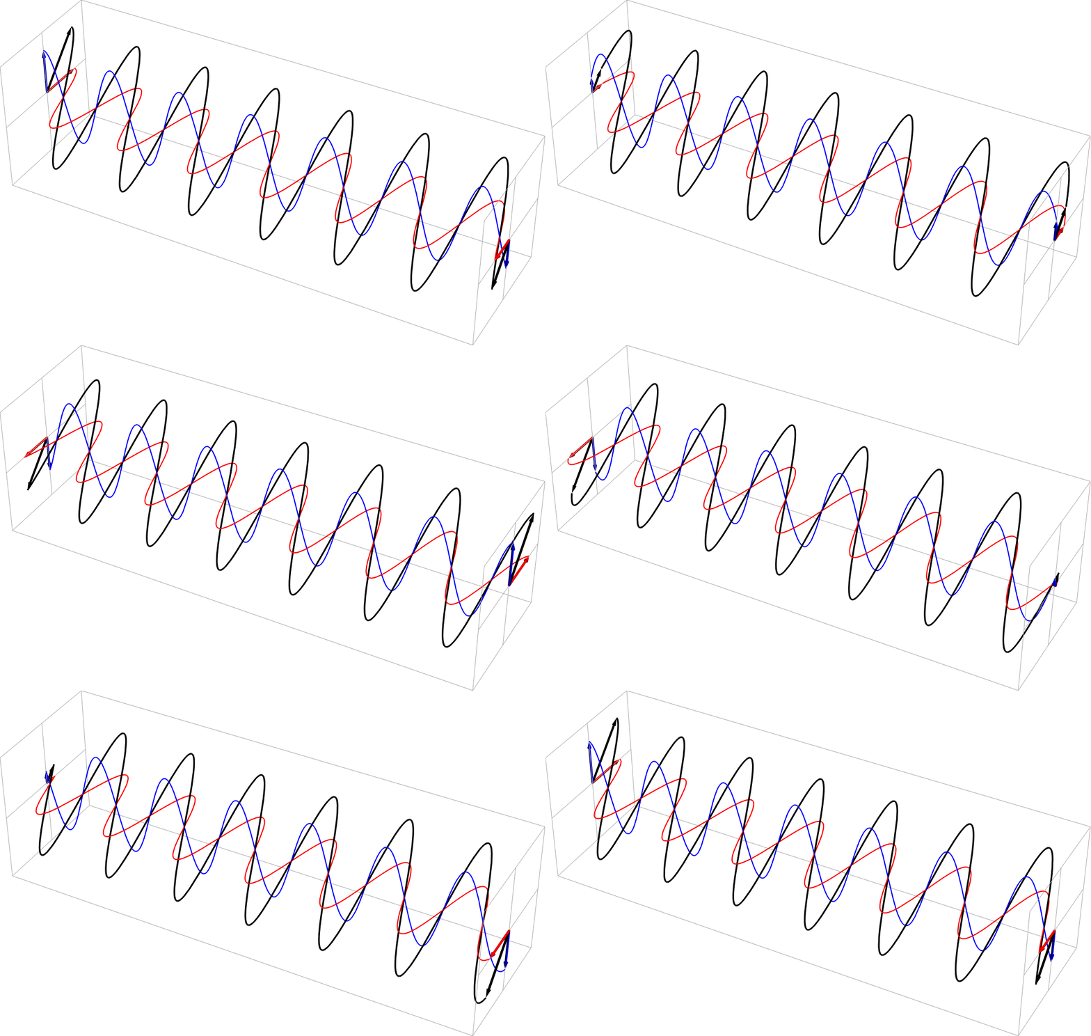
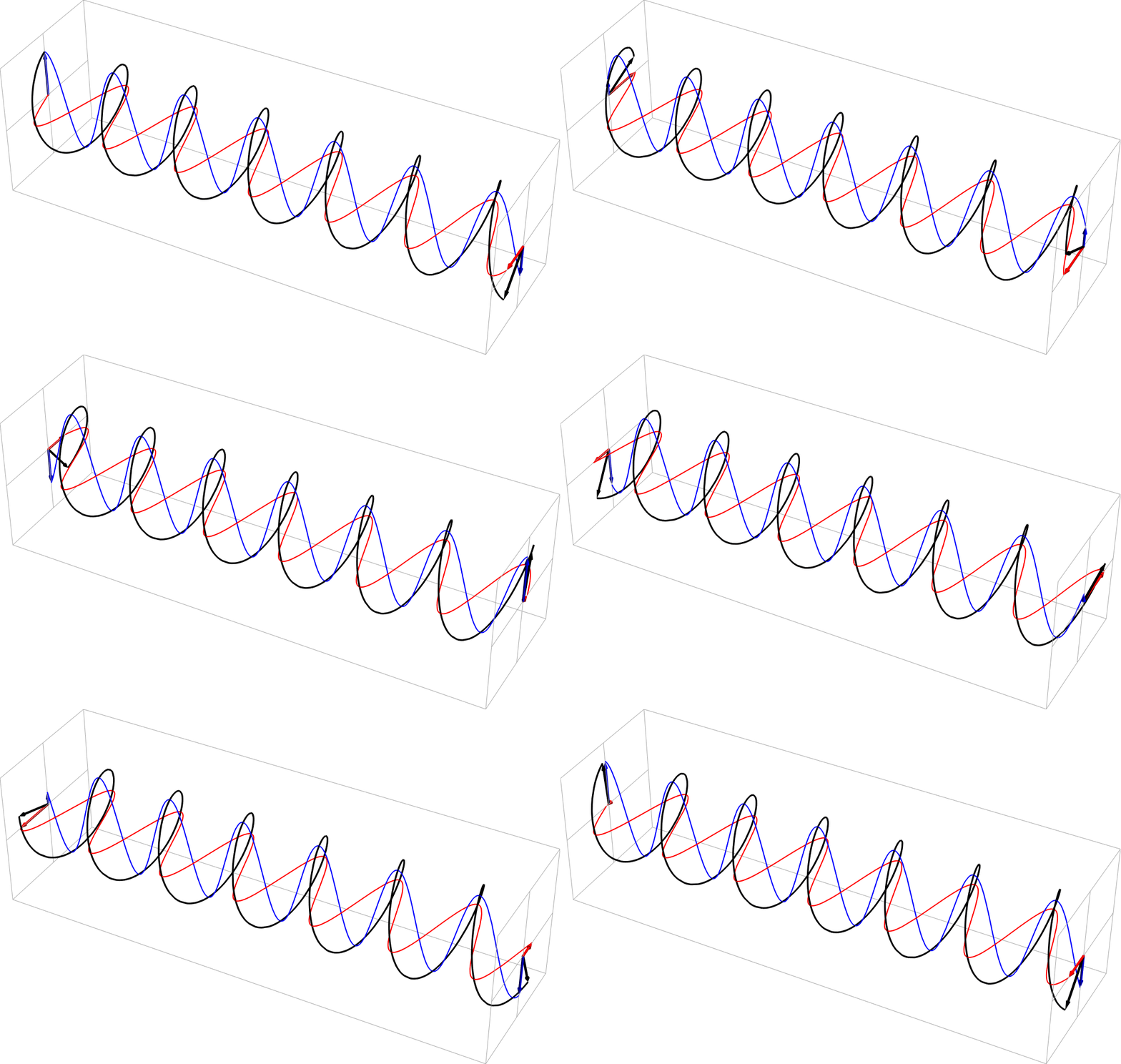
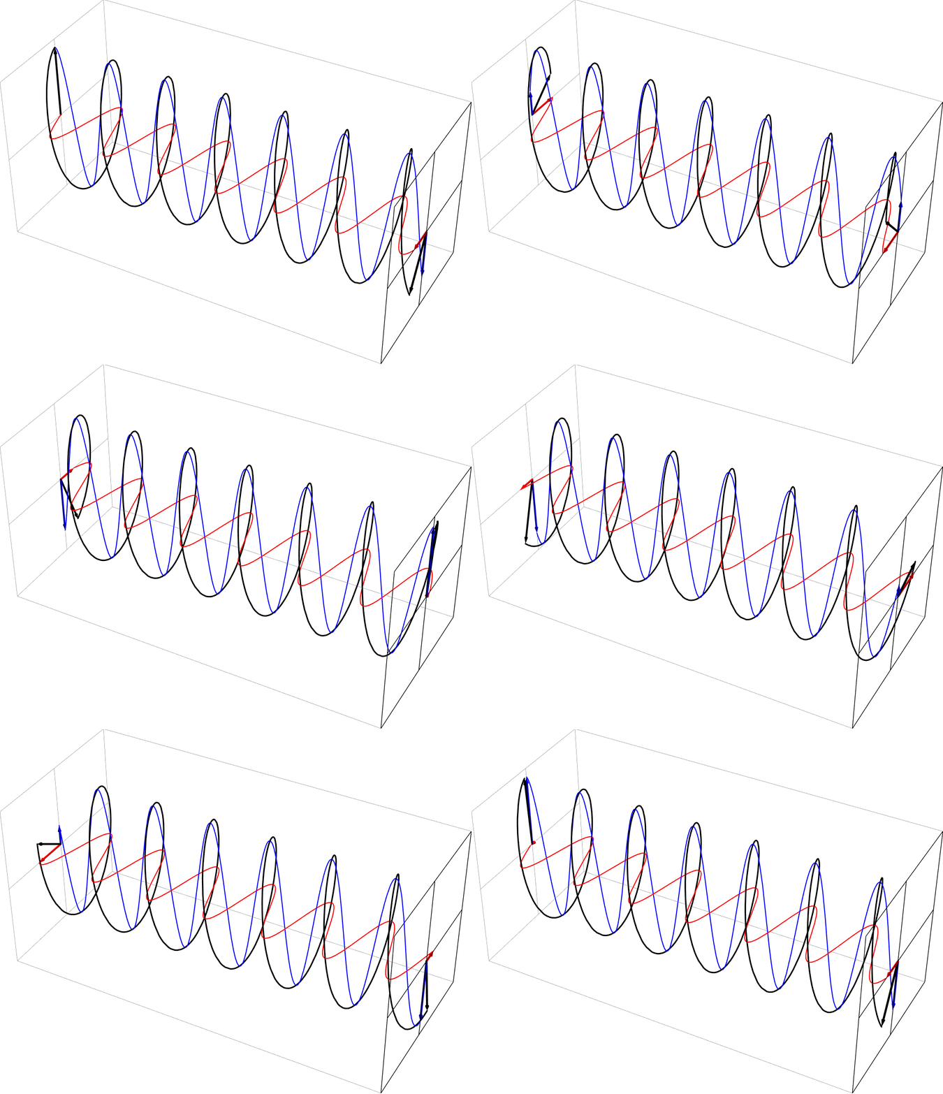
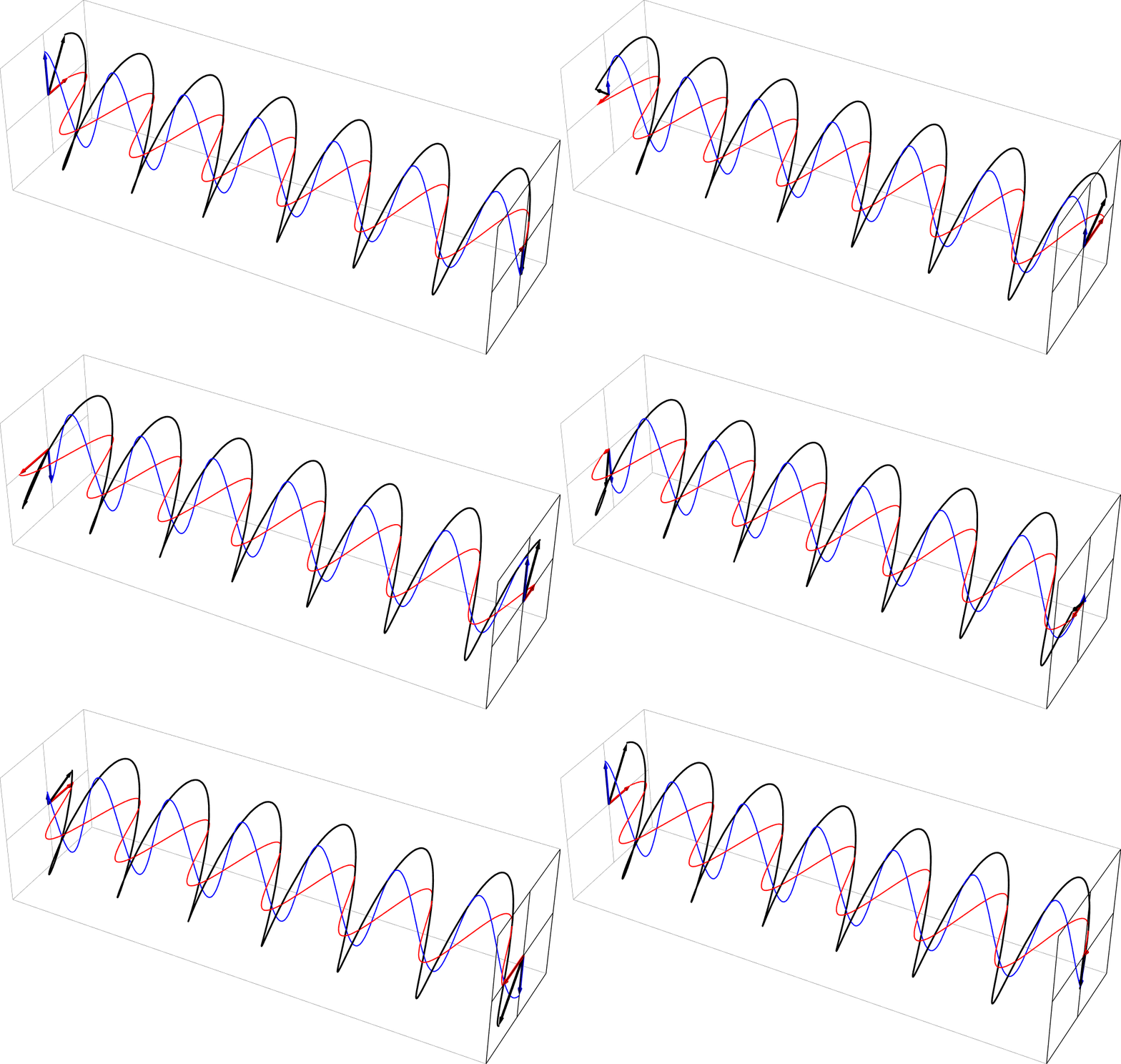
Here are some animations depicting how horizontally and vertically polarized light combine to produce other polarizations.
- Diagonal polarization as a sum of equal part in phase horizontal and vertical polarizations
- Circular polarization as a sum of equal part 90 deg out of phase horizontal and vertical polarizations. This is right circular, in the usual nomenclature.
- Elliptical polarization as a sum of unequal part 90 deg out-of-phase horizontal and vertical polarizations (vertical = 2x horizontal). This is right-handed, in the usual nomenclature.
- Elliptical polarization as a sum of equal part -45 deg out-of-phase horizontal and vertical polarizations. This is left-handed, in the usual nomenclature.
- These polarization animations were all created with this Mathematica program which you're welcome to download (thanks to former student Levi Homer): Polarization-animation.nb
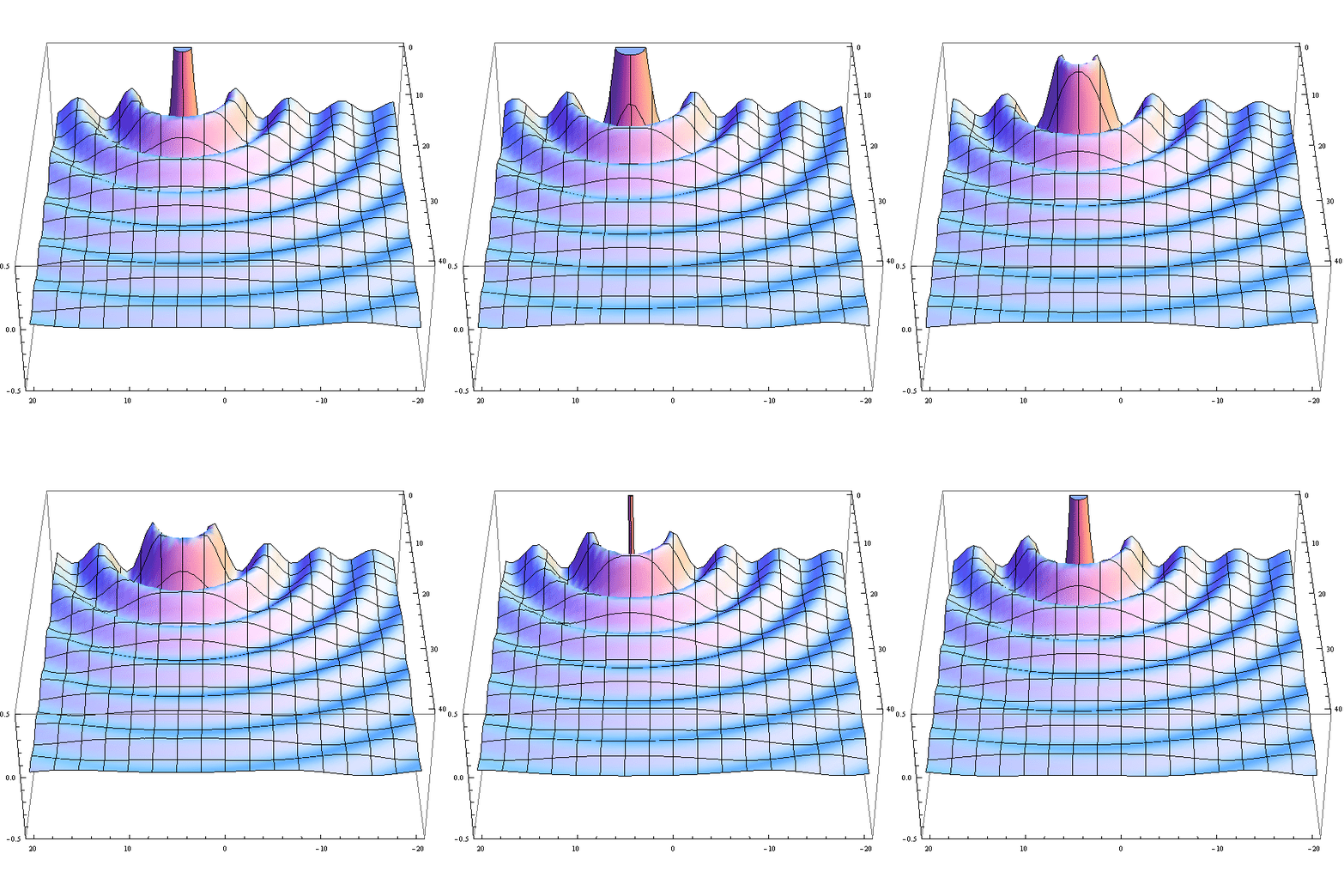
Here are depictions of spherical waves from point sources.
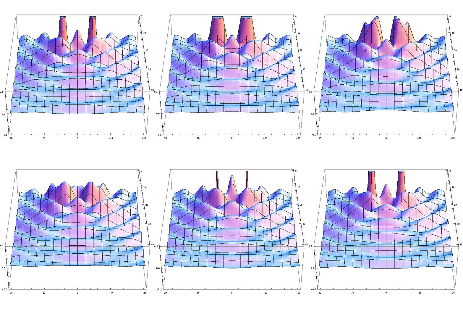
Here's an animation illustrating the Rayleigh criterion by plotting the sum of two jinc^2 functions.